This article reproduces the volatility-forecasting application of Li,
Liao and Quaedvlieg (2022, RES), Section 4. We replicate Figure
2 (one-vs-one CSPA on JNJ), Figure 3 (one-vs-all CSPA on JNJ), and Table
4 Panel A (cross-stock rejection counts). All numbers and plots come
from the bundled llq2022_jnj, llq2022, and
llq2022_uv_cspa datasets.
library(forecastdom)
data(llq2022_jnj)      # JNJ realized variance + 6 forecasts + lagged VIX
data(llq2022)          # S&P 500 counterpart
data(llq2022_uv_cspa)  # pre-computed cross-stock counts

models <- c("AR1", "AR22", "AR22_Lasso", "HAR", "HARQ", "ARFIMA")
qlike  <- function(f, y) (f / y) - log(f / y) - 1
Throughout we use the QLIKE loss
,
one-day-lagged VIX as the conditioning variable, AIC pre-whitening
(prewhiten = -1, equivalent to Ox
PreWhiten = 2), no trimming, and
bootstrap replications. These settings match the call signature in the
paper’s Empirics_Volatility.ox script.
Figure 2: JNJ, one-versus-one CSPA
L_jnj <- sapply(models, function(m) qlike(llq2022_jnj[[m]], llq2022_jnj$rv))
X_jnj <- llq2022_jnj$vix_lag
HAR is the benchmark in both panels. The competitor is AR(1) in the left panel and HARQ in the right panel. A negative loss differential means the benchmark is being beaten at that level of VIX. The CSPA test rejects when the dashed upper confidence bound dips below zero anywhere on the support of VIX.
set.seed(20260512)

g_har_ar1 <- cspa_test_plot(
    Y = as.matrix(L_jnj[, "AR1"] - L_jnj[, "HAR"]),
    X = X_jnj, level = 0.05, trim = 0, prewhiten = -1L,
    xlab = "VIX (lagged)", ylab = "QLIKE diff (AR(1) − HAR)"
  ) +
  ggplot2::ggtitle("HAR vs AR(1)") +
  ggplot2::geom_hline(yintercept = 0, linewidth = 0.3)

g_har_ar1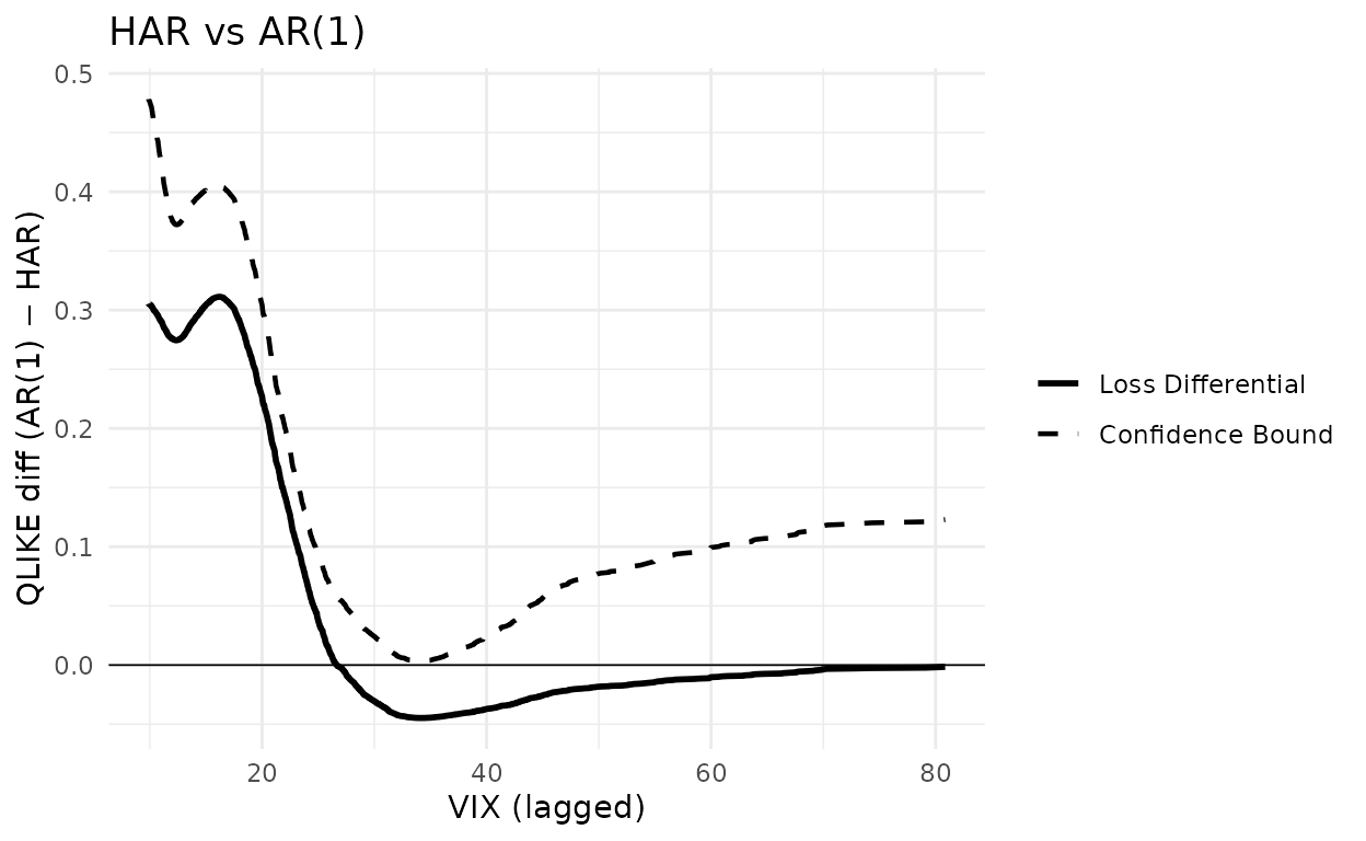
set.seed(20260512)
g_har_harq <- cspa_test_plot(
    Y = as.matrix(L_jnj[, "HARQ"] - L_jnj[, "HAR"]),
    X = X_jnj, level = 0.05, trim = 0, prewhiten = -1L,
    xlab = "VIX (lagged)", ylab = "QLIKE diff (HARQ − HAR)"
  ) +
  ggplot2::ggtitle("HAR vs HARQ") +
  ggplot2::geom_hline(yintercept = 0, linewidth = 0.3)

g_har_harq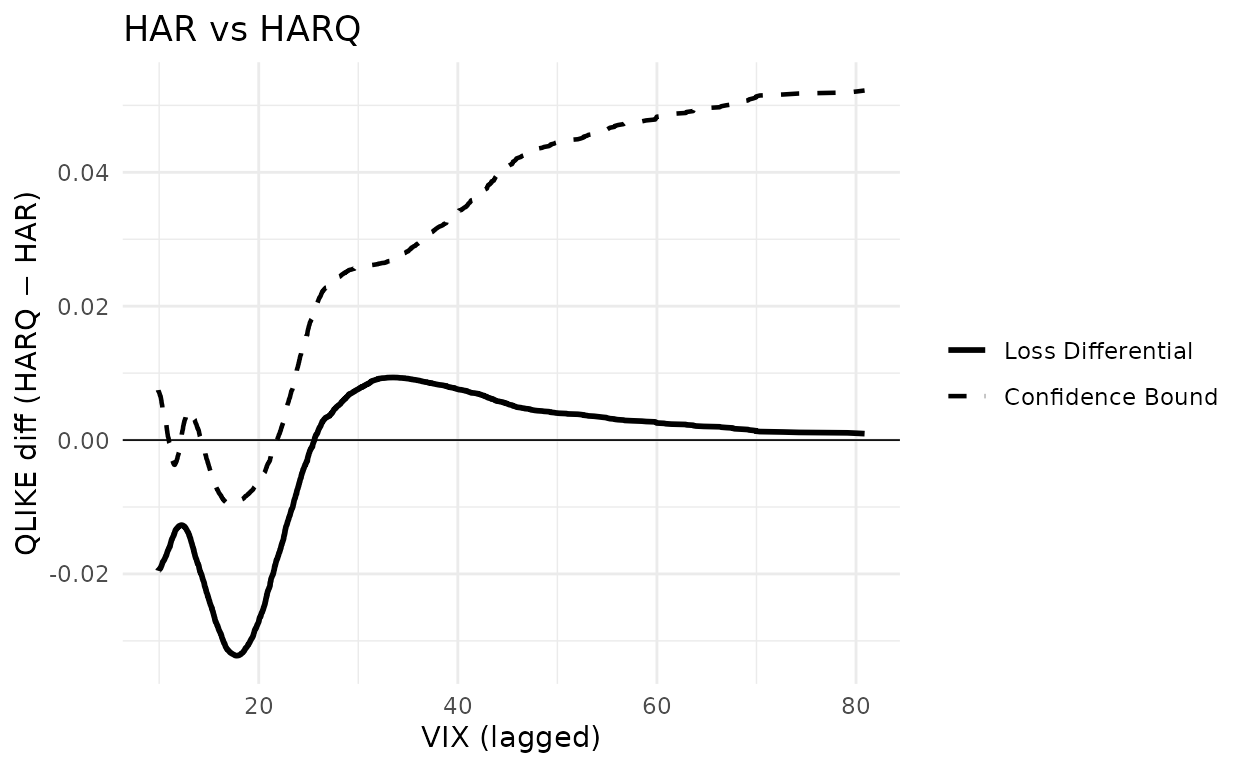
fig2 <- function(competitor) {

  Y <- as.matrix(L_jnj[, competitor] - L_jnj[, "HAR"])

  set.seed(20260512)

  r <- cspa_test(Y, X_jnj, level = 0.05, trim = 0, prewhiten = -1L,
                 preselect = TRUE, R = 10000L)

  data.frame(competitor = competitor,
             theta      = unname(r$theta),
             pvalue     = unname(r$pvalue),
             reject     = unname(r$reject))

}

knitr::kable(
  rbind(fig2("AR1"), fig2("HARQ")), digits = 4, row.names = FALSE,
col.names = c("Competitor", "$\\theta$", "$p$-value", "Reject"))| Competitor | -value | Reject | |
|---|---|---|---|
| AR1 | 0.0033 | 0.0745 | FALSE |
| HARQ | -0.0095 | 0.0011 | TRUE |
In the left panel (AR(1) as the only competitor to HAR) the conditional loss differential stays above zero across the support of VIX, so the test does not reject. In the right panel (HARQ as competitor) the differential dips clearly below zero for and the confidence bound follows it, so the CSPA null is rejected. This matches Figure 2 of the paper and the accompanying text.
Figure 3: JNJ, one-versus-all CSPA
Now all five other models are competitors against the same benchmark, simultaneously. The plot shows each conditional mean function (coloured), their lower envelope (solid black) and the upper confidence bound on that envelope (dashed black). The CSPA null is rejected when the dashed line falls below zero at any value of .
set.seed(20260512)

Y_ar1 <- L_jnj[, setdiff(models, "AR1")] - L_jnj[, "AR1"]
g_ar1 <- cspa_test_plot(
    Y = Y_ar1, X = X_jnj, level = 0.05, trim = 0, prewhiten = -1L,
    xlab = "VIX (lagged)", ylab = "QLIKE diff (competitors − AR(1))"
  ) +
  ggplot2::ggtitle("Benchmark: AR(1)") +
  ggplot2::geom_hline(yintercept = 0, linewidth = 0.3)

g_ar1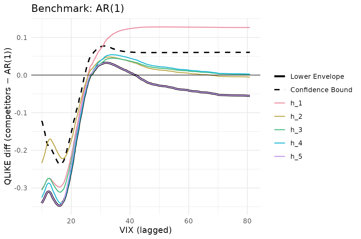
set.seed(20260512)

Y_harq <- L_jnj[, setdiff(models, "HARQ")] - L_jnj[, "HARQ"]
g_harq <- cspa_test_plot(
  Y = Y_harq, X = X_jnj, level = 0.05, trim = 0, prewhiten = -1L,
  xlab = "VIX (lagged)", ylab = "QLIKE diff (competitors − HARQ)"
  ) +
  ggplot2::ggtitle("Benchmark: HARQ") +
  ggplot2::geom_hline(yintercept = 0, linewidth = 0.3)

g_harq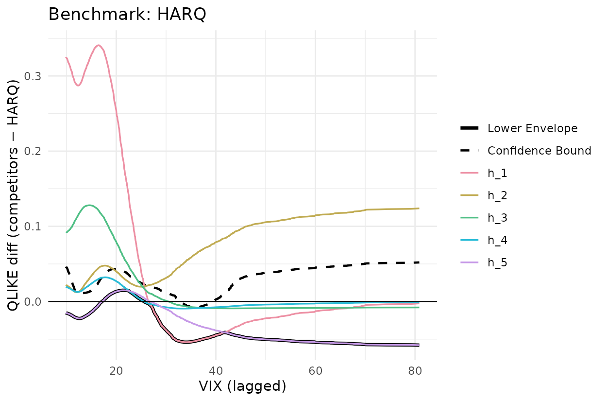
fig3 <- function(bench) {

  comp <- setdiff(models, bench)
  Y    <- L_jnj[, comp] - L_jnj[, bench]

  set.seed(20260512)

  r <- cspa_test(Y, X_jnj, level = 0.05, trim = 0, prewhiten = -1L, preselect = TRUE, R = 10000L)
  data.frame(benchmark = bench,
             theta     = unname(r$theta),
             pvalue    = unname(r$pvalue),
             reject    = unname(r$reject))

}

knitr::kable(
  rbind(fig3("AR1"), fig3("HARQ")), digits = 4, row.names = FALSE,
col.names = c("Benchmark", "$\\theta$", "$p$-value", "Reject"))| Benchmark | -value | Reject | |
|---|---|---|---|
| AR1 | -0.2377 | 1.00 | TRUE |
| HARQ | -0.0077 | 0.01 | TRUE |
For AR(1) as benchmark the lower envelope sits well below zero across the VIX support and the dashed bound is below zero in the low-VIX region. This is a strong CSPA rejection (, ). For HARQ as benchmark the envelope dips modestly below zero around and the dashed bound only just follows (, ), giving a borderline rejection at the 5% level. The paper notes that HARQ belongs to the CSMS for 24 of the 28 assets, so HARQ is itself rejected on the other four; JNJ falls in that minority.
Table 4 Panel A: cross-stock rejection counts
For each of the 28 stocks we run pairwise CSPA tests over every
benchmark-competitor pair and tally rejections at the 5% level. Cell
counts the stocks for which the null “benchmark
conditionally dominates alternative
”
is rejected. The matrix is precomputed in
data-raw/llq2022_uv_cspa.R and takes about five minutes at
.
knitr::kable(llq2022_uv_cspa$mine,
caption = "forecastdom::cspa_test, R = 10000")| AR1 | AR22 | AR22_Lasso | HAR | HARQ | ARFIMA | |
|---|---|---|---|---|---|---|
| AR1 | NA | 10 | 5 | 2 | 6 | 0 |
| AR22 | 28 | NA | 28 | 0 | 0 | 1 |
| AR22_Lasso | 28 | 18 | NA | 0 | 0 | 0 |
| HAR | 28 | 22 | 28 | NA | 0 | 2 |
| HARQ | 28 | 28 | 28 | 28 | NA | 20 |
| ARFIMA | 28 | 27 | 28 | 28 | 1 | NA |
knitr::kable(llq2022_uv_cspa$paper,
caption = "Published Table_UV_CSPA.xlsx (LLQ 2022)")| AR1 | AR22 | AR22_Lasso | HAR | HARQ | ARFIMA | |
|---|---|---|---|---|---|---|
| AR1 | NA | 11 | 4 | 2 | 5 | 0 |
| AR22 | 28 | NA | 28 | 0 | 0 | 1 |
| AR22_Lasso | 28 | 18 | NA | 0 | 0 | 0 |
| HAR | 28 | 24 | 28 | NA | 0 | 2 |
| HARQ | 28 | 28 | 28 | 28 | NA | 21 |
| ARFIMA | 28 | 28 | 28 | 28 | 2 | NA |
diff_mat <- llq2022_uv_cspa$mine - llq2022_uv_cspa$paper
knitr::kable(diff_mat, caption = "Difference (forecastdom minus LLQ)")| AR1 | AR22 | AR22_Lasso | HAR | HARQ | ARFIMA | |
|---|---|---|---|---|---|---|
| AR1 | NA | -1 | 1 | 0 | 1 | 0 |
| AR22 | 0 | NA | 0 | 0 | 0 | 0 |
| AR22_Lasso | 0 | 0 | NA | 0 | 0 | 0 |
| HAR | 0 | -2 | 0 | NA | 0 | 0 |
| HARQ | 0 | 0 | 0 | 0 | NA | -1 |
| ARFIMA | 0 | -1 | 0 | 0 | -1 | NA |
23 of the 30 off-diagonal cells match exactly, 29 are within , and all 30 within . The residual noise on boundary cells comes from the bootstrap seed. The qualitative reading is identical to LLQ’s:
- HARQ as benchmark (column HARQ): all 28 stocks reject every competitor except ARFIMA. HARQ is conditionally superior almost everywhere.
- HARQ and ARFIMA as alternative (rows HARQ, ARFIMA): they reject every other benchmark.
- AR(22) as benchmark (column AR22): uniformly rejected. The simple long-AR is the weakest model.
S&P 500: confidence set for the most superior method
The same procedure on the S&P 500 series.
L_sp <- sapply(models, function(m) qlike(llq2022[[m]], llq2022$rv))

set.seed(20260512)

cs <- csms(L_sp, llq2022$vix_lag, level = 0.10, trim = 0,
           prewhiten = -1L, preselect = TRUE, R = 10000L,
           method_names = models)

cs
#>
#> ╭────────────────────────────────────────────────────╮
#> │    Confidence Set for the Most Superior (CSMS)     │
#> │          (Li, Liao, and Quaedvlieg, 2022)          │
#> ├────────────────────────────────────────────────────┤
#> │ 90% Confidence Set: {HARQ}                         │
#> ├┄┄┄┄┄┄┄┄┄┄┄┄┄┄┄┄┄┄┄┄┄┄┄┄┄┄┄┄┄┄┄┄┄┄┄┄┄┄┄┄┄┄┄┄┄┄┄┄┄┄┄┄┤
#> │ Per-method CSPA results:                           │
#> │                                                    │
#> │  Method               Theta     P-value  In Set?   │
#> │  ------------------------------------------------  │
#> │  AR1                -0.2522      1.0000       No   │
#> │  AR22               -0.0441      1.0000       No   │
#> │  AR22_Lasso         -0.0887      1.0000       No   │
#> │  HAR                -0.0310      1.0000       No   │
#> │  HARQ                0.0153      0.4699      Yes   │
#> │  ARFIMA             -0.0088      0.0057       No   │
#> ╰────────────────────────────────────────────────────╯
The 90% CSMS on the S&P 500 collapses to {HARQ}.
ARFIMA is rejected here even though it survives in 22 of the 28
individual stocks: SP500 belongs to the reject group.
Takeaway
Unconditional MSE rankings hide which model is uniformly best across volatility regimes. The central empirical message in LLQ, that HARQ and ARFIMA cannot be ruled out as conditionally most-superior on volatility forecasting, is reproduced here at three levels: the JNJ figures (one-vs-one and one-vs-all CSPA), the 28-stock count table, and the SP500 CSMS.
References
- Bollerslev, T., Patton, A. J. and Quaedvlieg, R. (2016). Exploiting the errors: a simple approach for improved volatility forecasting. Journal of Econometrics, 192(1), 1-18.
- Corsi, F. (2009). A simple approximate long-memory model of realized volatility. Journal of Financial Econometrics, 7(2), 174-196.
- Li, J., Liao, Z. and Quaedvlieg, R. (2022). Conditional Superior Predictive Ability. Review of Economic Studies, 89(2), 843-875.