Get Started with forecastdom • forecastdom

Overview

forecastdom collects forecast evaluation tests under the taxonomy of Li, Liao, and Quaedvlieg (2022):

	Equal accuracy	Superior accuracy
Unconditional	`dm_test()`	`spa_test()`
Conditional	`gw_test()`	`cspa_test()`

It also bundles the tests usually paired with these in applied work: nested-model comparisons (cw_test(), enc_new(), mse_f_test()), return predictability (ivx_wald()), and parameter instability (qll_hat()).

library(forecastdom)
set.seed(42)

Pairwise Forecast Comparison

Diebold-Mariano test

Compares two sets of forecast errors and asks whether the average loss differential is zero.

e1 <- rnorm(200)
e2 <- rnorm(200, mean = 0.15)

dm_test(e1, e2)
#> 
#> ╭────────────────────────────────────────────────────╮
#> │     Modified Diebold-Mariano Test (HLN, 1997)      │
#> ├────────────────────────────────────────────────────┤
#> │ H0: Equal predictive ability                       │
#> │ H1: Methods have different predictive ability      │
#> ├┄┄┄┄┄┄┄┄┄┄┄┄┄┄┄┄┄┄┄┄┄┄┄┄┄┄┄┄┄┄┄┄┄┄┄┄┄┄┄┄┄┄┄┄┄┄┄┄┄┄┄┄┤
#> │ Test Results:                                      │
#> │  DM statistic: 0.2073                              │
#> │  P-value: 0.8360                                   │
#> ├┄┄┄┄┄┄┄┄┄┄┄┄┄┄┄┄┄┄┄┄┄┄┄┄┄┄┄┄┄┄┄┄┄┄┄┄┄┄┄┄┄┄┄┄┄┄┄┄┄┄┄┄┤
#> │ Details:                                           │
#> │  Observations (n): 200                             │
#> │  Forecast horizon (h): 1                           │
#> │  Loss function: SE                                 │
#> │  Reference distribution: t(199)                    │
#> ╰────────────────────────────────────────────────────╯

The default correction = TRUE applies the Harvey, Leybourne, and Newbold (1997) small-sample correction, which uses a $t$ distribution with $T - 1$ degrees of freedom in place of the asymptotic normal.

Clark-West test

The standard DM test is undersized when the two models are nested. The Clark-West (2007) MSFE-adjusted statistic fixes this by adding a correction term for the extra parameters in the larger model and is approximately $N(0,1)$ under the null.

actual <- rnorm(200)
f1 <- actual + rnorm(200, sd = 0.5) # benchmark (restricted)
f2 <- actual + rnorm(200, sd = 0.4) # alternative (unrestricted)

cw_test(actual - f1, actual - f2, f1, f2)
#> 
#> ╭────────────────────────────────────────────────────╮
#> │               Clark-West Test (2007)               │
#> ├────────────────────────────────────────────────────┤
#> │ H0: Benchmark MSFE <= Alternative MSFE             │
#> │ H1: Alternative model is superior (R2OS > 0)       │
#> ├┄┄┄┄┄┄┄┄┄┄┄┄┄┄┄┄┄┄┄┄┄┄┄┄┄┄┄┄┄┄┄┄┄┄┄┄┄┄┄┄┄┄┄┄┄┄┄┄┄┄┄┄┤
#> │ Test Results:                                      │
#> │  CW statistic: 9.1803                              │
#> │  P-value (one-sided): 0.0000                       │
#> │  R2OS (%): 10.18                                   │
#> ├┄┄┄┄┄┄┄┄┄┄┄┄┄┄┄┄┄┄┄┄┄┄┄┄┄┄┄┄┄┄┄┄┄┄┄┄┄┄┄┄┄┄┄┄┄┄┄┄┄┄┄┄┤
#> │ Details:                                           │
#> │  Observations (n): 200                             │
#> │  Reference distribution: N(0,1)                    │
#> ╰────────────────────────────────────────────────────╯

Giacomini-White test

Asks whether two methods have equal predictive ability given the information available to the forecaster. The default instruments are a constant and the lagged loss differential.

gw_test(e1, e2)
#> 
#> ╭────────────────────────────────────────────────────╮
#> │     Conditional Equal Predictive Ability Test      │
#> │            (Giacomini and White, 2006)             │
#> ├────────────────────────────────────────────────────┤
#> │ H0: Equal conditional predictive ability           │
#> │ H1: Methods differ conditionally                   │
#> ├┄┄┄┄┄┄┄┄┄┄┄┄┄┄┄┄┄┄┄┄┄┄┄┄┄┄┄┄┄┄┄┄┄┄┄┄┄┄┄┄┄┄┄┄┄┄┄┄┄┄┄┄┤
#> │ Test Results:                                      │
#> │  Wald statistic: 1.3426                            │
#> │  P-value: 0.5110                                   │
#> ├┄┄┄┄┄┄┄┄┄┄┄┄┄┄┄┄┄┄┄┄┄┄┄┄┄┄┄┄┄┄┄┄┄┄┄┄┄┄┄┄┄┄┄┄┄┄┄┄┄┄┄┄┤
#> │ Details:                                           │
#> │  Observations (n): 199                             │
#> │  Instruments (q): 2                                │
#> │  Loss function: SE                                 │
#> │  Reference distribution: Chi-sq(2)                 │
#> ╰────────────────────────────────────────────────────╯

Multiple Forecast Comparison

Hansen’s SPA test

Asks whether the benchmark has the lowest expected loss among all competitors. The null is that no competitor beats the benchmark on average; the bootstrap controls family-wise error across the $J$ comparisons.

sim <- do_sim(J = 3, n = 250, a = 1, c = 0, rho_u = 0.4)
spa_test(sim$Y, level = 0.05, B = 1000)
#> 
#> ╭────────────────────────────────────────────────────╮
#> │          Superior Predictive Ability Test          │
#> │                   (Hansen, 2005)                   │
#> ├────────────────────────────────────────────────────┤
#> │ H0: Benchmark is superior to all competitors       │
#> │ H1: Some competitor outperforms the benchmark      │
#> ├┄┄┄┄┄┄┄┄┄┄┄┄┄┄┄┄┄┄┄┄┄┄┄┄┄┄┄┄┄┄┄┄┄┄┄┄┄┄┄┄┄┄┄┄┄┄┄┄┄┄┄┄┤
#> │ Test Results:                                      │
#> │  SPA statistic: 50.4916                            │
#> │  P-value (bootstrap): 0.0020                       │
#> │  Decision: Rejected ***                            │
#> ├┄┄┄┄┄┄┄┄┄┄┄┄┄┄┄┄┄┄┄┄┄┄┄┄┄┄┄┄┄┄┄┄┄┄┄┄┄┄┄┄┄┄┄┄┄┄┄┄┄┄┄┄┤
#> │ Details:                                           │
#> │  Observations (n): 250                             │
#> │  Competitors (J): 3                                │
#> │  Bootstrap replications: 1000                      │
#> │  Significance level: 0.0500                        │
#> ╰────────────────────────────────────────────────────╯

CSPA test

Li, Liao, and Quaedvlieg (2022) ask the same question conditional on a state variable $X_t$ . The null is

$H_0:\ \min_{j}\, \mathbb{E}[L_{0,t} - L_{j,t} \mid X_t = x] \le 0 \quad \text{for all } x,$

i.e. there is no competitor and no state value where the benchmark is strictly worse. The test combines a Legendre-polynomial series estimate of the conditional mean differentials $h_j(x)$ with an HAC-based Gaussian-process critical value.

# Under the null (a = 1) the benchmark is weakly dominant
sim_null <- do_sim(J = 3, n = 500, a = 1, c = 0, rho_u = 0.4)
cspa_test(sim_null$Y, sim_null$X, level = 0.05, trim = 2)
#> 
#> ╭────────────────────────────────────────────────────╮
#> │      Conditional Superior Predictive Ability       │
#> │          (Li, Liao, and Quaedvlieg, 2022)          │
#> ├────────────────────────────────────────────────────┤
#> │ H0: Benchmark weakly dominates all competitors     │
#> │     conditionally, uniformly across all states     │
#> │ H1: Some competitor outperforms the benchmark      │
#> │     in certain conditioning states                 │
#> ├┄┄┄┄┄┄┄┄┄┄┄┄┄┄┄┄┄┄┄┄┄┄┄┄┄┄┄┄┄┄┄┄┄┄┄┄┄┄┄┄┄┄┄┄┄┄┄┄┄┄┄┄┤
#> │ Test Results:                                      │
#> │  Theta: 0.1488                                     │
#> │  P-value: 0.4666                                   │
#> │  Significance level: 0.0500                        │
#> │  Decision: Not rejected                            │
#> ├┄┄┄┄┄┄┄┄┄┄┄┄┄┄┄┄┄┄┄┄┄┄┄┄┄┄┄┄┄┄┄┄┄┄┄┄┄┄┄┄┄┄┄┄┄┄┄┄┄┄┄┄┤
#> │ Estimation Details:                                │
#> │  Observations (n): 480                             │
#> │  Competitors (J): 3                                │
#> │  Series terms (K): 4                               │
#> │  HAC lag order: 1 (pre-whitened)                   │
#> │  Selected (j,x) pairs: 1440 / 1440 (100.0%)        │
#> ╰────────────────────────────────────────────────────╯

# Under the alternative (a = 1.5) one competitor beats the benchmark in some states
sim_alt <- do_sim(J = 3, n = 500, a = 1.5, c = 0, rho_u = 0.4)
result <- cspa_test(sim_alt$Y, sim_alt$X, level = 0.05, trim = 2)

result
#> 
#> ╭────────────────────────────────────────────────────╮
#> │      Conditional Superior Predictive Ability       │
#> │          (Li, Liao, and Quaedvlieg, 2022)          │
#> ├────────────────────────────────────────────────────┤
#> │ H0: Benchmark weakly dominates all competitors     │
#> │     conditionally, uniformly across all states     │
#> │ H1: Some competitor outperforms the benchmark      │
#> │     in certain conditioning states                 │
#> ├┄┄┄┄┄┄┄┄┄┄┄┄┄┄┄┄┄┄┄┄┄┄┄┄┄┄┄┄┄┄┄┄┄┄┄┄┄┄┄┄┄┄┄┄┄┄┄┄┄┄┄┄┤
#> │ Test Results:                                      │
#> │  Theta: -0.2217                                    │
#> │  P-value: 0.0002                                   │
#> │  Significance level: 0.0500                        │
#> │  Decision: Rejected ***                            │
#> ├┄┄┄┄┄┄┄┄┄┄┄┄┄┄┄┄┄┄┄┄┄┄┄┄┄┄┄┄┄┄┄┄┄┄┄┄┄┄┄┄┄┄┄┄┄┄┄┄┄┄┄┄┤
#> │ Estimation Details:                                │
#> │  Observations (n): 480                             │
#> │  Competitors (J): 3                                │
#> │  Series terms (K): 4                               │
#> │  HAC lag order: 1 (pre-whitened)                   │
#> │  Selected (j,x) pairs: 1440 / 1440 (100.0%)        │
#> ╰────────────────────────────────────────────────────╯

Visualization

cspa_test_plot() draws the estimated conditional means $\hat h_j(x)$ , their lower envelope, and the upper confidence bound on that envelope. The CSPA null is rejected when the dashed bound drops below zero anywhere on the support of $x$ .

cspa_test_plot(result)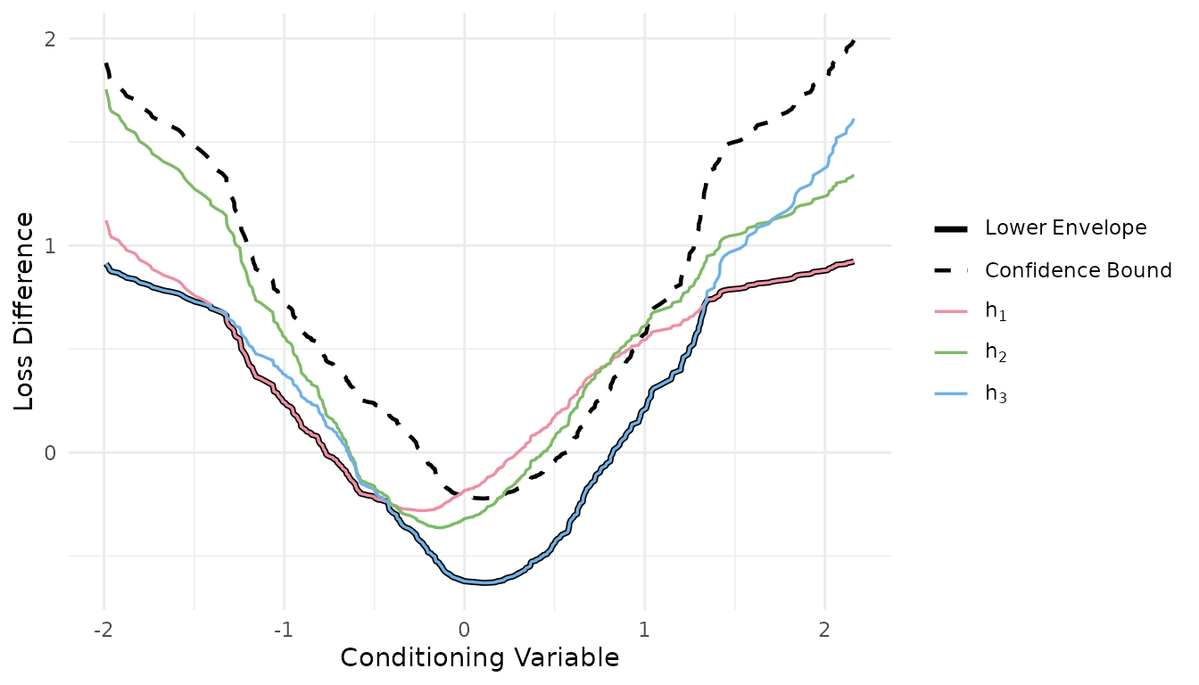

CSMS: confidence set for the most superior

If no model is singled out as the benchmark, csms() runs the CSPA test once per candidate and keeps the candidates that are not rejected. The resulting set is asymptotically a level- $(1-\alpha)$ confidence set for the conditionally most-superior method.

csms(losses, X, level = 0.05, trim = 2, method_names = c("AR1", "HAR", "HARQ", "LASSO"))

Predictive Regressions

IVX-Wald test

Kostakis, Magdalinos, and Stamatogiannis (2015) build an instrument from a near-stationary transformation of the regressor so that the predictability test has a standard $\chi^2$ distribution even when the predictor is near-unit-root.

n <- 300
x <- cumsum(rnorm(n))
y <- 0.02 * x + rnorm(n)

ivx_wald(y, as.matrix(x), K = 1, M_n = floor(n^(1/3)))
#> 
#> ╭────────────────────────────────────────────────────╮
#> │      IVX-Wald Test for Predictive Regressions      │
#> │  (Kostakis, Magdalinos, and Stamatogiannis, 2015)  │
#> ├────────────────────────────────────────────────────┤
#> │ H0: No predictability (all coefficients = 0)       │
#> │ H1: At least one predictor is significant          │
#> ├┄┄┄┄┄┄┄┄┄┄┄┄┄┄┄┄┄┄┄┄┄┄┄┄┄┄┄┄┄┄┄┄┄┄┄┄┄┄┄┄┄┄┄┄┄┄┄┄┄┄┄┄┤
#> │ Test Results:                                      │
#> │  IVX-Wald statistic: 13.4596                       │
#> │  P-value: 0.0002                                   │
#> ├┄┄┄┄┄┄┄┄┄┄┄┄┄┄┄┄┄┄┄┄┄┄┄┄┄┄┄┄┄┄┄┄┄┄┄┄┄┄┄┄┄┄┄┄┄┄┄┄┄┄┄┄┤
#> │ Details:                                           │
#> │  Observations (T): 300                             │
#> │  Predictors (r): 1                                 │
#> │  Forecast horizon (K): 1                           │
#> │  Reference distribution: Chi-sq(1)                 │
#> ├┄┄┄┄┄┄┄┄┄┄┄┄┄┄┄┄┄┄┄┄┄┄┄┄┄┄┄┄┄┄┄┄┄┄┄┄┄┄┄┄┄┄┄┄┄┄┄┄┄┄┄┄┤
#> │ IVX Coefficients:                                  │
#> │    beta_1: 0.0249                                  │
#> ╰────────────────────────────────────────────────────╯

Elliott-Muller test

Tests $H_0:\ \beta_t = \beta$ for all $t$ against the alternative that the regression coefficient drifts. The statistic $\widehat{qLL}$ has a non-standard limit; critical values are tabulated in Elliott and Muller (2006, Table 1).

X <- matrix(rnorm(n * 2), n, 2)
y2 <- X %*% c(0.5, -0.3) + rnorm(n)

qll_hat(y2, X, L = floor(n ^ (1 / 3)))
#> 
#> ╭────────────────────────────────────────────────────╮
#> │ Elliott-Muller Test for Time-Varying Coefficients  │
#> │             (Elliott and Muller, 2006)             │
#> ├────────────────────────────────────────────────────┤
#> │ H0: Constant coefficients (beta(t) = beta)         │
#> │ H1: Time-varying coefficients                      │
#> ├┄┄┄┄┄┄┄┄┄┄┄┄┄┄┄┄┄┄┄┄┄┄┄┄┄┄┄┄┄┄┄┄┄┄┄┄┄┄┄┄┄┄┄┄┄┄┄┄┄┄┄┄┤
#> │ Test Results:                                      │
#> │  qLL-hat statistic: -7.2358                        │
#> │  5% critical value: -10.64                         │
#> │  Decision (5%): Not rejected                       │
#> ├┄┄┄┄┄┄┄┄┄┄┄┄┄┄┄┄┄┄┄┄┄┄┄┄┄┄┄┄┄┄┄┄┄┄┄┄┄┄┄┄┄┄┄┄┄┄┄┄┄┄┄┄┤
#> │ Details:                                           │
#> │  Observations (T): 300                             │
#> │  Time-varying coefficients (k): 2                  │
#> │ Note: Non-standard distribution.                   │
#> │ Reject when qLL-hat < critical value.              │
#> ╰────────────────────────────────────────────────────╯

References

Clark, T.E. and McCracken, M.W. (2001). Tests of Equal Forecast Accuracy and Encompassing for Nested Models. Journal of Econometrics, 105(1), 85-110.
Clark, T.E. and West, K.D. (2007). Approximately Normal Tests for Equal Predictive Accuracy in Nested Models. Journal of Econometrics, 138(1), 291-311.
Diebold, F.X. and Mariano, R.S. (1995). Comparing Predictive Accuracy. Journal of Business & Economic Statistics, 13(3), 253-263.
Elliott, G. and Muller, U.K. (2006). Efficient Tests for General Persistent Time Variation in Regression Coefficients. Review of Economic Studies, 73(4), 907-940.
Giacomini, R. and White, H. (2006). Tests of Conditional Predictive Ability. Econometrica, 74(6), 1545-1578.
Hansen, P.R. (2005). A Test for Superior Predictive Ability. Journal of Business & Economic Statistics, 23(4), 365-380.
Harvey, D., Leybourne, S., and Newbold, P. (1997). Testing the Equality of Prediction Mean Squared Errors. International Journal of Forecasting, 13(2), 281-291.
Kostakis, A., Magdalinos, T., and Stamatogiannis, M.P. (2015). Robust Econometric Inference for Stock Return Predictability. Review of Financial Studies, 28(5), 1506-1553.
Li, J., Liao, Z., and Quaedvlieg, R. (2022). Conditional Superior Predictive Ability. Review of Economic Studies, 89(2), 843-875.